What is Catastrophe Theory and some relevant aspects of Catastrophe Theory is discussed.  The application of Catastrophe Theory to developmental research through the method of catastrophe detection, catastrophe analysis and catastrophe modelling is described.  The catastrophe theoretical approach as a potential tool for studying conceptual development, specifically the development of the concept of matter and its transformations, in science education and its implications is also considered.

INTRODUCTION

The concept of stages in cognitive development (Piaget & Inhelder, 1969) has come to dominate the field of education through its far-reaching educational implications.  However, the debate and controversy concerning empirical criteria and methods for detecting stages and the subsequent interpretation of the results obtained continues unabated.  Fischer (1983) voices this anxiety, “... Would they (developmental researchers) be able to detect the stage that was right there in front of them ?  If they did notice it, how would they know what they had found ?  How would they be able to tell that it was a stage ?  What pattern of results would they look for ?”  It was then concluded that developmental researchers do not have a uniform empirical criterion to determine the existence of a stage.

Stage criteria such as invariant sequences, cognitive structure, integration, consolidation and equilibration has been proposed by Piaget (1960) while transition criteria such as bimodality, sudden spurts, response variability and second-order transitions has been pointed out by Flavell(1971).  Unfortunately, such stage and transition criteria have seldom been investigated simultaneously.  In addition to this, the rationale for each criterion was not derived from an explicit formal transition theory (van der Maas & Molenaar, 1992).

Connell and Furman (1984) propose that all the transition criteria ought to be integrated within a formal model.  This is because empirical evidence on the basis of any one transition criteria is insufficient to support or reject the Piagetian Stage hypothesis.  A basic formal theoretical model of transition criteria would enable the integration of empirical evidence for stage transitions into a powerful argument for stagewise development.  Such a formal model may be obtained through a branch of mathematics called Catastrophe Theory (Thom, 1975).

Catastrophe Theory

The term “Catastrophe Theory” first appeared in the western press in the late sixties.  It was hailed as “a revolution in mathematics, comparable perhaps to Newton’s invention of the differential and integral calculus” (Arnol’d, 1992).  Catastrophe Theory was applied with great diversity to areas such as the study of heart beat, geometrical and physical optics, embryology, linguistics, experimental psychology, economics, hydrodynamics, geology and the theory of elementary particles.

The founder of Catastrophe Theory was René Thom.  The origins of Catastrophe Theory may be traced to Whitney’s theory of singularities of smooth mappings and Poincaré and Andronov’s theory of bifurcations of dynamical systems. Singularities, bifurcations and catastrophes are different terms used to describe the emergence of discrete structures from smooth and continuous ones.  Singularity theory is a broad generalization of the study of functions at maximum and minimum points.  Bifurcation means forking and is used to designate all kinds of qualitative re-organizations or metamorphoses of various entities as a result of a change in the parameters on which they depend.  Catastrophes are abrupt changes which arise as a sudden response of a system to a smooth change in external conditions.

Catastrophe Theory provides a universal method for the study of all discontinuities, jump transitions and sudden qualitative changes.  Catastrophe Theory involves the study of the equilibrium behaviour of a large class of mathematical system functions that exhibit discontinuous jumps, that is, the points of the functions where at least the first and second derivatives are zero.  The mathematical theorems of Catastrophe Theory constitute an essential contribution to the study of the singularities of families of smooth functions or infinitesimally differentiable functions.

Some aspects of Catastrophe Theory

Stagewise or stage-by-stage development entails the concepts of stage and transition.  Catastrophe Theory is capable of describing physical systems with a well-defined discontinuity.  For example, boiling, which involves a transition between the liquid phase and the gaseous phase of water.  Catastrophe Theory, which is part of a nonlinear dynamic system theory, may be used to model such physical systems.  Such dynamic models are of sufficient complexity to transcend the dichotomy between the organismic and mechanistic paradigms (Molenaar & Oppenheimer, 1985).  As a result, Catastrophe Theory has been successfully applied in psychological perception research (Stewart & Peregoy, 1983; Taéed, Taéed & Wright, 1988) and clinical psychology (Callahan & Sashin, 1990).

Models derived from Catastrophe Theory relates behavioural (dependent) variables to control (independent) variables.  Discontinuities in behavioural variables is modelled as a function of continuous variation in the control variables.  The relationship between behavioural and control variables is in the form of mathematical expressions which represent a dynamical system which is continually seeking to reach equilibrium in varying situations.  For certain fixed values of the control variables, the behavioural variable will change optimally until a stable state is attained.

The models obtained through Catastrophe Theory is also subject to a basic principle of mathematical modelling, that is, the hypothesis of structural stability or insensitivity to small perturbations.  This hypothesis states that there is some kind of overall stability in any mathematical model of a real system.  This stability corresponds to the inherent stability of observable phenomena in the real world.  Therefore, there is the notion of stable equilibrium for a dynamical system.  A dynamical system is some process which evolves continuously with time.  The system is changing slowly due to changes in various parameters which describe the system.  The equilibrium also changes and becomes less and less stable until for a particular value or values of the parameters, the equilibrium becomes unstable and disappears altogether.  Consequently, the behaviour of the system would also undergo a sudden switch from one equilibrium state to another.  The dynamical system with a continuous input thus produces a sudden discontinuity in its output.

Thom (1975) was able to show that for a certain fairly common kind of dynamical system, the various ways in which these discontinuous jumps in output occur may be described geometrically.  It was further proven that a large class of structurally stable system functions (involving up to four control variables) exhibiting discontinuous behaviour may be classified into seven archetypical forms (the elementary catastrophe models) through a set of smooth transformations of the system variables.  The catastrophe models are the fold, the cusp, the swallow-tail, the elliptic umbilic or hair, the hyperbolic umbilic or breaking wave, the butterfly and the parabolic umbilic or the mushroom.  The most popular elementary catastrophe model is the cusp.  All structurally system functions which show discontinuous behaviour in three dimensions may be transformed to a cusp.

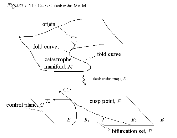
The Cusp Catastrophe Model

The cusp catastrophe is denoted by

  V (x)  =  ¼ x 4  +  ½ c1   x 2  +  c2   x ...... (1)

where c1  and c2  are the control parameters (or independent variables) and x is the behavioural variable (or dependent variable).  Critical points occur where  V1 (x)  =  0 , that is,

   x3   +  c1  x  +  c2   =  0           .......... (2)

and they coalesce where V 11  (x)  =  0 , that is,

   3x2   +  c1   =  0                         .......... (3)

Eliminating x gives

   4c1  3   +  27 c2  2   =  0           .......... (4)

for the equation of the catastrophe set  K.
          The complex behaviour of the function (that is, the relationship between x,  c1  , c2  ) may be elucidated in a very revealing way by representing it geometrically in three dimensions.  This is done by drawing the associated catastrophe manifold or equilibrium surface of points in the  (x,  c1  , c2 )-space.  This space is the set  M of points (x,  c1  , c2 ) which satisfies Equation 2.  The catastrophe manifold, M, has the appearance of a folded smooth surface as shown in Figure1.

        A clearer picture of this folded surface may be obtained from an analysis of the catastrophe map X  :  M         C  which projects points on M onto the  ( c1  , c2  ) - plane or the control plane, C, according to ( x,  c1  , c2  )           ( c1  , c2  )   where x  c  M  in the neighbourhood of the origin.  This projection in the control plane C is a semicubical parabola denoted by Equation 4, which is the equation of the catastrophe set  K.
        The control plane may be divided into five subsets : the shaded region  I   ‘inside’ the curve, the region  E  ‘outside’ it, the two branches B1   and  B2   of the curve and the origin P.  The points ( c1  , c2  ) which lie in  I  are those for which  4c1  3   +  27 c2  2   < 0 , those in E satisfy  4c1  3   +  27 c2  2   >  0  and those on the curve satisfy  4c1  3   +  27 c2  2   =  0.
        It is now possible to give a geometrical interpretation of the nature of the equilibria of the dynamical system.  For a given pair of control parameters ( c1  , c2  ), the equilibria are obtained by solving Equation 1.  The roots may be described as the x-coordinates of the points at which a vertical through ( c1  , c2  ) meets the catastrophe manifold, M.  Geometrically, it may be seen that
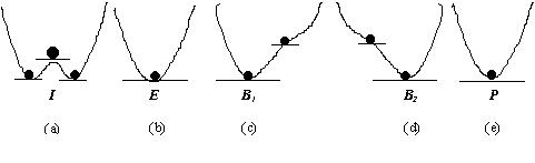
If  ( c1  , c2  ) lies in the region  I , that is, where 4c1  3   +  27 c2  2   < 0 ,  there are three distinct real roots.  This means that there are three values of x since there are three “sheets” of M  lying above points in  I .  This particular region in the control plane,  C , is called the bifurcation set,  B .   V  takes the form shown in Figure 2(a), that is, two minima on either side of a maximum.
If  ( c1  , c2  )  lies  in  the  region  E  external  to  the  bifurcation set  B,   that  is, where      4c1  3   +  27 c2  2   >  0 , there is one real root.  This means that there is a unique value of x since only one sheet of  M lies above points in  E .  The cusp function  V  takes the form shown in Figure 2(b), that is, a minimum.
If  ( c1  , c2  )  lies on  B1  , that is, where  4c1  3   +  27 c2  2   =  0 , there are three real roots; two of which are equal, with the equal pair being larger.  This means that there are three values of x (of which two are equal and larger than the third).  The vertical line through          ( c1  , c2  ) passes through the lower sheet at a single point and is tangential to the upper sheet.  The cusp function  V  takes the form shown in Figure 2(c), that is, a minimum and a point of inflexion to the right of the minimum.
If  ( c1  , c2  ) lies on  B2  , that is, where   4c1  3   +  27 c2  2   =  0 , there are three real roots; two of which are equal, with the equal pair being smaller.  This means that there are three values of  x  (of which two are equal and smaller than the third).  The vertical line through  ( c1  , c2  ) is tangential to the lower sheet and passes through the upper sheet at a single point.  The cusp function  V  takes the form shown in Figure 2(d), that is, a minimum and a point of inflexion to the left of the minimum.
If   ( c1  , c2  )  lies on the cusp point,  P , that is, where  c1   =  c2    =  0 ,  there are three real coincident roots (all equal to 0).  This means that there are three values of  x  which are coincident and equal zero since the vertical line through ( c1  , c2  ) is tangential to the surface M  and meets it at a single point, the origin, which passes through three sheets of  M ;  all at the same point.  The cusp function,  V , takes the form shown in Figure 2(e), that is, a minimum.

Minima of  V  correspond to stable equilibrium while maxima or points of inflexion correspond to unstable equilibria.  Hence, for control parameters in  , B1  , B2   and  P ,  there is a single equilibrium whereas for control parameters in  I  (that is, the bifurcation set), there are two stable equilibria and one unstable equilibrium.  In other words, unstable equilibria correspond to points on  M  lying inside the fold curve on the middle of the three sheets while stable equiria lie outside the fold curve.

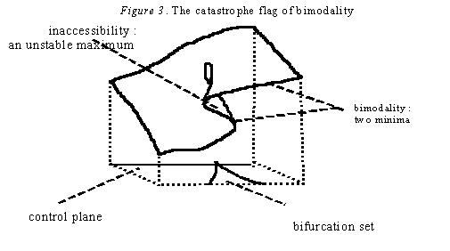
In the bifurcation set, three modes of behaviour are possible.  The middle sheet represents unstable states and is therefore called the inaccessible region.  The presence of the two remaining modes implies a bimodal distribution of the behavioural variable.  Phenomena such as bimodality can be used as an indicator of discontinuities.  It is called a catastrophe flag by Gilmore (1981) and can be used to detect catastrophes.

The Application of Catastrophe Theory to Stagewise Development

The Catastrophe Theory approach to stagewise development may be carried out through three methods :  catastrophe detection, catastrophe analysis and catastrophe modelling.

Catastrophe Detection

Catastrophe Theory yields a set of mathematically derived criteria to detect discontinuities or catastrophes.  Gilmore (1981) refers to these criteria as catastrophe flags.  Catastrophe detection provides empirical evidence for transitions in development.  The occurrence of a catastrophe is invariantly associated with catastrophe flags which can be used as an indicator of discontinuities.  Catastrophe flags include bimodality, inaccessibility, sudden jumps, hysteresis and divergence.  The detection of catastrophe flags is quite straightforward as only behavioural measures are required.  Catastrophe detection is especially useful in the initial analysis of stagewise development.  These flags can be used to detect stage-to-stage transitions.

Modality relates to the properties of bimodal score distributions.  There are three modes of behaviour possible in the bifurcation set.  The maximum is not a stable state and is called the inaccessible region.  The remaining two modes, represented by minima, implies a bimodal distribution of the behavioural variable.  This is shown in Figure 3 and Figure 4.

According to Wohlwill (1973), the occurrence of a sharp bimodal distribution of scores may be due to the high degree of interdependence among responses to different items of a test.  This is indicative of discontinuous behaviour.  In contrast, if the various items are independent, a uniform or normal distribution would be obtained due to continuous change.  In other words, a discontinuity in cognitive level as a function of age may be translated directly into a distribution of scores.  It follows then that intermediate test scores will be low in proportion.

The catstrophe flag of sudden jumps or spurts is directly coupled to bimodality and inaccessibilty.  It is also a property of transitions.  A sudden jump is defined as a large change in the value of the behavioural variable because of a small change in the value of a control variable.  Such spurts in developmental functions may be detected using a developmental test (the yardstick) and age (the clock) for cognitive change.  Fischer (1983) discussed a number of applications of this method in different fields such as speech development, brain development, object performance and classification.

Hysteresis refers to jumps at distinct values of the control variables when these control variables follow either an increasing or decreasing path.  Hysteresis may be difficult to detect as the actual control variables have to be known in order to be manipulated effectively (that is, experimentally induced to continuous increase or decrease).  Hysteresis has been successfully detected in simple neural networks that may be relevant to simulation of stagewise development (van der Maas, Verschure & Molenaar, 1990).

Divergence occurs when a small change in the initial value of a path through the control plane leads to large changes in the behavioural variable.  Fischer, Pipp and Bullock (1984) suggest that optimality of environmental test conditions control the discontinuity in the manner represented by the splitting control variable.  Change along this splitting control variable will lead to divergence of the two modes of behaviour.

The five catastrophe flags of bimodality, inaccessibilty, sudden jumps, hysteresis and divergence occur simultaneously when the system is in transition.  They occur when the values of the control variables are inside the bifurcation set.

Catastrophe Analysis

Catastrophe analysis involves analysing mathematically the dynamic equations which describe a transition process.  These equations are repeatedly subjected to certain transformation techniques to reduce them to one of the seven archetypical or original geometrical forms specified by Thom (1975), that is, the elementary catastrophe models.  Hence, catastrophe analysis requires a knowledge of the mathematical equations of the transition process.

The use of catastrophe analysis has been demonstrated in the physical sciences (Poston & Stewart, 1978).  However, this variant of Catastrophe Theory is hindered in the social sciences due to the lack of knowledge of the precise dynamical equations governing the types of transitions explored.  In fact, determination of the control variables of such transitions is also an obstacle.  This is because discontinuities in psychological behaviour may be the result of simple discontinuous change in the independent variables and not the variables which actually controls the behaviour (that is, the control variables).  This necessitates the restriction to continuous variation of the control variables as only the control variables could bring about intrinsic reorganization which constitutes a genuine stage transition.

Catastrophe Modelling

Catastrophe modelling is intermediate in strength between catastrophe detection and catastrophe analysis.  Catastrophe modelling involves the direct specification of behavioural and control variables in one of the elementary catastrophes.

The Conflict Cusp Model, proposed by van der Maas and Molenaar (1990), relates discontinuities in conservation acquisition to the set of different strategies for solving conservation items by an appeal to the concept of cognitive conflict.

The behavioural variable, denoted by p, is defined by the quotient of the number of correct judgements of conservation items and the total number of conservation items.  The test score is thus given by chance level, for example, p = 1 or 0 or 0.5.  The control variables are based on conservation strategies which are classified into three types : conservation strategies (CS), nonconservation strategies (NS) and irrelevant strategies (IS).  A conserver will use mainly CS and IS while a nonconserver will use NS and IS.  Transitional children will have at their disposal all three types of conservation strategies whereas the remaining children (the residual group) will use predominantly IS.  The Conflict Cusp Model is shown in Figure 5.

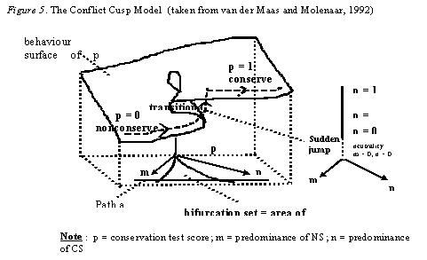
Discontinuities can occur when both control variables are active, that is, m and n are high.  A typical stage transition is illustrated by Path a.  First, a nonconserver consistently uses NS.  Therefore, the test score depends only on m and will be below chance level (that is, p = 0.5).  With increase in the value of n corresponding to a predominance of CS, the child reaches the bifurcation set and becomes transitional.  Both CS and NS are now available and the child is faced with a situation often described as a cognitive conflict (Cantor, 1983; Pinard, 1981).  The middle sheet of the cusp represents a situation in which both CS and NS have equal influence.  However, this region is inaccessible and consists of unstable states.  This means that a transitional child will score either below or above chance level but not at the chance level.  Hence, even though both predominances are equally strong, the actual application of strategies (and therefore the test scores) is biased towards only one set of strategies.  On leaving the bifurcation set, the jump to a higher level takes place and the child becomes a stable conserver.

The conservation score of both conservers and nonconservers is continuously related to variation in predominances of CS and NS (or the values of m and n).  Variation along the m-axis (that is, n = 0) corresponding to variation in the predominance of NS in nonconservers yields continuous changes in the test score.  Variation along the n-axis (that is, m = 0) corresponding to variation in the predominance of CS in conservers will also yield continuous changes in the test score.  When the values of m and n are both high, sudden jumps or transitions occur for the transitional group.  The residual group is placed around the neutral point where both predominances are equal.  The use of IS by these groups yields scores at the chance level. This model has not been tested empirically.

Catastrophe modelling concerns the actual fitting of the model to data which requires statistical techniques.  Strong evidence for the presence of a stage transition is indicated by a goodness of fit of a catastrophe model which is statistically acceptable.

Conclusion

Catastrophe Theory provides a means to mathematically analyse the dynamics of nonlinear systems.  Catastrophes mark transitions to newly emerging equilibria that is the result of endogenous reorganization or self-organization of the system dynamics.

According to van der Maas and Molenaar (1992), catastrophes constitute formal analogues of stage transitions in Piaget’s theory of cognitive development.  This is because the human cognitive system is one of the most complex information-processing systems in nature.  Cognitive development may be characterised in a formal sense as the evolution of a nonlinear dynamic system in which the mathematical results of Catastrophe Theory are obeyed.  The Catastrophe Theory approach to stagewise development as proposed by van der Maas and Molenaar (1992) gives to a straightforward methodology for detecting and modelling stage transitions.  Empirical research in catastrophe detection and catastrophe modelling comprise a definite test for stage transitions.

Even though the catastrophe theoretical approach was originally a formal approach to cognitive development, it cannot be denied that this approach is feasible for other forms of development, in particular the development of science concepts for students in science education.  The comprehension of science concepts and its subsequent application in new situations is a form of development which requires very specific input.  For example, the concept of matter and its transformations is very fundamental with ever-widening application as the study of science progresses.  It is also very abstract as it involves the conceptualization of matter as being particulate and dynamic and capable of interacting with other particles.  The necessary instruction such as the Particle and Kinetic Theory of Matter definitely has to be imparted to students as it is not “something that is in the air” which students will ultimately absorb with increasing experience and maturity.  Formal instruction is required and teachers need to take students over the boundary between their haphazard and mainly narcissistic beliefs which are the result of everyday experiences to the realm of scientific knowledge.

Hence, instruction in the concept of matter and its transformations is a very probable control variable in students’ conceptual development of matter and its transformations.  Research towards the determination of the exact control variables and the precise nature of this conceptual development will be invaluable in the sense that catastrophes in conceptual development of students could be customized.  This holds promise for science instruction and the school science curriculum.  If it can be envisaged that certain input or instruction could bring about a catastrophe or an abrupt major re-organization in the understanding of a science concept, then appropriate re-structuring of the curriculum may be better directed and more relevant.  This could lead the way to the development of science concepts as a planned part of the curriculum.

References

Arnol’d, V. I. (1992).  Catastrophe theory. New York : Springer-Verlag.
Callahan, J., & Sashin, J. I. (1990).  Predictive  models  in  psychoanalysis. Behavioural Science,  33, 97-115.
Cantor, G. N. (1983). Conflict,  learning  and  Piaget  :  Comments  on  Zimmerman  and  Blom’s  “Toward  an  empirical
    test  of the role of cognitive conflict in learning”. Developmental   Review, 3, 39-53.
Connell, J. P., & Furman, W. (1984).  The  study of  transitions : Conceptual and methodological  issues.  In  R. N. Emde  &   R. J.  Harmon  (Eds.),    Continuities  and  discontinuities  in  development (pp. 153-174). New York : Plenum Press.
Fischer, K. W. (1993).  Developmental levels as periods of discontinuity.  In K. W. Fischer (Ed.).  Levels and transitions
    in children’s development: New directions for child development  (Vol. 21, pp. 5-20). San Francisco : Jossey-Bass.
Fischer, K. W.,   Pipp, S. L.,  &  Bullock, D. (1984).  Detecting  developmental  discontinuities :  methods  and
    measurement.  In  R. N.  Emde  & R. J.  Harmon  (Eds.), Continuities and  discontinuities in development
    (pp. 95-122). New York : Plenum Press.
Flavell, J. H. (1971). Stage-related properties of cognitive development. Cognitive Psychology, 2,  421-453.
Gilmore, R. (1981). Catastrophe Theory for scientists and engineers. New York : Wiley.
Molenaar,  P. C. M.,  &  Oppenheimer,  L. (1985).   Dynamic  models  for  development  and  the  mechanistic-
    organismic controversy. New Ideas in Psychology, 3, 233-242.
Piaget,  J. (1960).  The general problems of the psychological development of the child.   In J. M.  Tanner &  B.
    Inhelder (Eds.),  Discussions  on  child  development,  (Vol. 4,  pp.  3-28).  London : Tavistock.
Piaget, J., & Inhelder, B. (1969). The psychology of the child. New York : Basic Books.
Pinard, A. (1981).  The conservation of conservation : The child’s acquisition of a fundamental  concept.  Chicago :
    University of Chicago Press.
Poston, T., & Stewart, I. (1978). Catastrophe theory and its applications. London : Pitman.
Stewart,  I.  N.,   &  Peregoy,  P.  L.  (1983).     Catastrophe  theory   modelling   in   psychology.  Psychological Bulletin,
    94, 336-362.
Taéed, L. K., Taéed, O., &  Wright, J. E. (1988).  Determinants involved in the perception of the  necker cube : An
    application of catastrophe theory. Behavioural Science, 33, 97-115.
Thom, R. (1975). Structural stability and morphogenesis. Reading, MA : Benjamin.
Van der Maas,  H. L. J.,  &  Molenaar,  P. C. M.  (1992).  Stagewise cognitive development : An  application of
    catastrophe theory. Psychological Review, 99 (3), 395-417.
Van der Maas,  H. L. J.,  Verschure, P. F. M.,  &  Molenaar,  P. C. M. (1990).  A note on chaotic  behaviour in simple
    neural networks. Neural Networks, 3, 119-122.
Wohlwill, J. F. (1973).  The  study  of   behavioural  development.  San Diego, CA  :  Academic  Press.

Kembali Ke Tajuk-Tajuk Kajian